가치관제작소

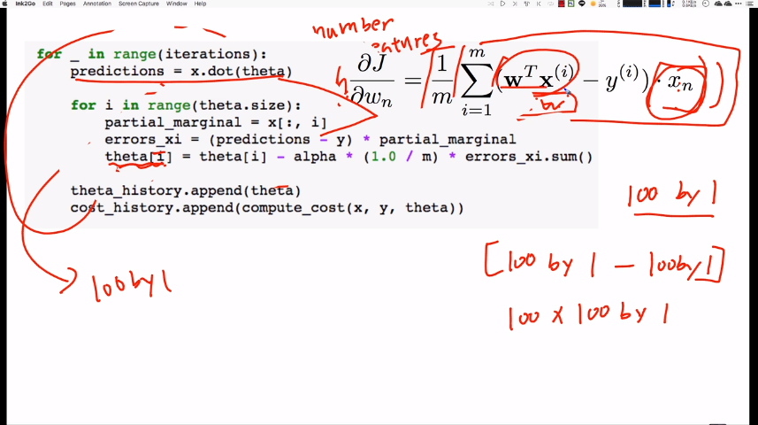
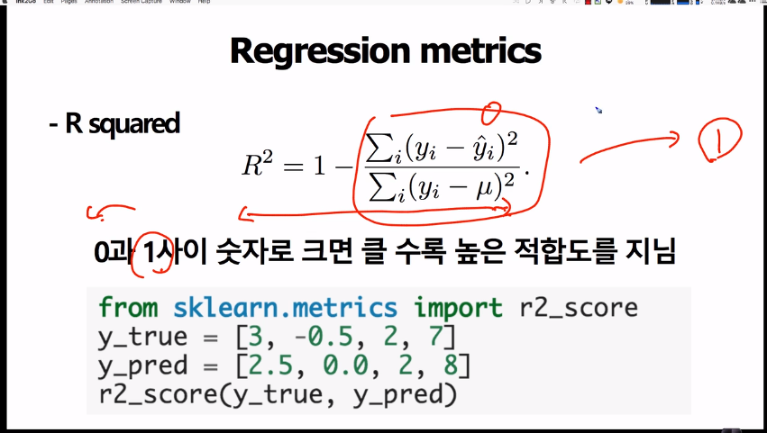
각 파라미터의 메트릭스, 벡터의 shape를 팔로우 하는 것이 이해에 중요하다.

raw_X가 (63,)데이타라고 할 때,

# [X] (63,2) matrix
# [Y] (63,) vector
# [w] (2,)vector
# [alpha] scalar

# [m] 트레이닝 데이터의 갯수 

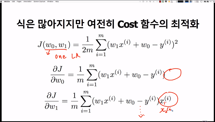
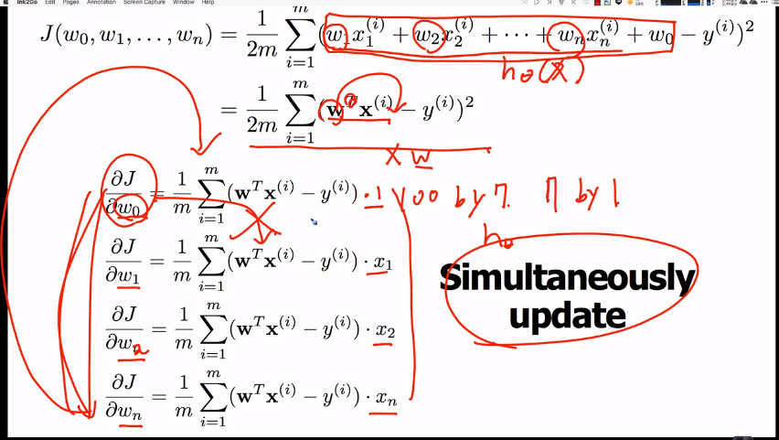
・n은 feature의 개수, m은 트레이닝 데이터의 개수

x[:10]  ➡(100,3)matrix

array([

[ 2.48270246, 2.20781622, 1. ],

[ 6.07241833, 9.19025007, 1. ],

[ 3.11546929, 4.64238367, 1. ],

[10.81785453, 3.26464437, 1. ],

[12.07014858, 4.42723458, 1. ],

[11.83337984, 5.07817642, 1. ],

[13.12434071, 10.7762702 , 1. ],

[ 9.89781386, 15.71398351, 1. ],

[10.00780438, 16.26077027, 1. ],

[17.19363062, 12.50682637, 1. ]])

y[:10]  ➡(100,)vector

array([533.83030493, 526.31007838, 532.42415066, 531.48943805, 533.43500502, 539.84331102, 535.17117282, 532.18836072, 541.13287791, 536.28514281])

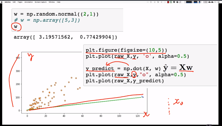
# predictions is (100, )vector by dot product.

Multivariate linear regression models

assignment

import numpy as np


class LinearRegressionGD(object):
    def __init__(self, fit_intercept=True, copy_X=True,
                 eta0=0.001, epochs=1000, weight_decay=0.9):
        self.fit_intercept = fit_intercept
        self.copy_X = copy_X
        self._eta0 = eta0
        self._epochs = epochs

        self._cost_history = []

        self._coef = None
        self._intercept = None
        self._new_X = None
        self._w_history = []
        self._weight_decay = weight_decay

        
        
    ######################
    # %function$ [cost]
    # %param$    [h] : numpy array, 2차원 matrix 형태로 [-1, n_predicted_targets]의 구조를 가진다.
    # %param$    [y] : numpy array, 실제 y 값을 1차원 vector 형태로 [n_real_values]의 구조를 가진다.
    # %return$   [cost_value] : cost_value : float형태의 scalar 값을 반환함
    ######################
    def cost(self, h, y):
#         y = y.reshape(-1,1)
#         cost_value  = (1/(2*len(y)))*(np.sum((h-y)**2))
#         return cost_value
        return (1/(2*len(y)))*(np.sum((h-y.reshape(-1,1))**2))
   

    ######################
    # %function$ [hypothesis_function]
    # %param$    [X] : numpy array, 2차원 matrix 형태로 [n_samples,n_features] 구조를 가진다
    # %param$    [theta] : numpy array, 가중치 weight값을 1차원 vector로 입력한다.
    # %return$   [Y_hat] : y_hat : numpy array, 예측된 값을 2차원 matrix 형태로 [-1, n_predicted_targets]의 구조를 가진다.
    ######################
    def hypothesis_function(self, X, theta):
#         y_hat = np.dot(X, theta)
#         y_hat = y_hat.reshape(-1,1)
        
#         return y_hat
    
        return np.dot(X, theta).reshape(-1,1)
    
    ######################
    # %function$ [cost]
    # %param$    [X] : numpy array, 2차원 matrix 형태로 [n_samples,n_features] 구조를 가진다
    # %param$    [y] : numpy array, 실제 y 값을 1차원 vector 형태로 [n_real_values]의 구조를 가진다.
    # %param$    [theta] : numpy array, 가중치 weight값을 1차원 vector로 입력한다.
    # %return$   [cost_value] : numpy array, 공식에 의해 산출된 gradient vector를 반환함.
    #                           이때 gradient vector는 weight의 갯수 만큼 element를 가진다.
    #                           반환되는 형태는 자유롭게 할 수 있으나 [-1, weight_gradient]나
    #                           weight_gradient]로 반환 후 다음 수식에서 사용하기 위한 처리가 필요하다.
    #                           현재는 벡터를 반환함
    ######################
    def gradient(self, X, y, theta):
        m = len(y)
        alpha = self._eta0
        y_prediction = np.dot(X,theta)
        
        for i in range(theta.size):
            theta[i] = theta[i] - (alpha/m) * np.sum((y_prediction - y) * X[:,i])
        
#         print(theta)
        return theta

    
    ######################
    # %function$ [fit]
    # %param$    [X] : numpy array, 2차원 matrix 형태로 [n_samples,n_features] 구조를 가진다
    # %param$    [y] : numpy array, 실제 y 값을 1차원 vector 형태로 [n_real_values]의 구조를 가진다.
    # %return$   [self]
    ######################
    def fit(self, X, y):
        # Write your code
        
        # if fit_intercept is true, create 1 as vector
        if(self.fit_intercept):
            x_rows =  X.shape[0]
            one_vector = np.ones(shape=(x_rows,1))
            X = np.hstack((one_vector, X))
            
        # save X to self._new_X
        self._new_X = X
        
        # initiate theta
        theta = np.ones(X.shape[1])

        # 1번의 full-batch가 데이터 전량을 사용하므로, 1epoch이라 할 수 있다.
        # 여기선 epoch을 iteration이라고 생각하면 편하다.
        for epoch in range(self._epochs):
            # 아래 코드를 반드시 활용할 것
            gradient = self.gradient(self._new_X, y, theta).flatten()

            # cotrol learning rate
            self._eta0 = self._eta0 * self._weight_decay
            
            # Write your code

            if epoch % 100 == 0:
                self._w_history.append(theta)
                cost = self.cost(self.hypothesis_function(self._new_X, theta), y)
                self._cost_history.append(cost)
            
        # Write your code
        self._coef = theta[1:,]
        self._intercept = theta[0]
        
#         print('#####################theta[1:,]',theta[1:,])
#         print('#####################theta[0]',theta[0])
#         print(self._w_history)
        
        return self


    ######################
    # %function$ [hypothesis_function]
    # %param$    [X] : numpy array, 2차원 matrix 형태로 [n_samples,n_features] 구조를 가진다
    # %param$    [theta] : numpy array, 가중치 weight값을 1차원 vector로 입력한다.
    # %return$   [Y_hat] : y_hat : numpy array, 예측된 값을 2차원 matrix 형태로 [-1, n_predicted_targets]의 구조를 가진다.
    ######################
    def predict(self, X):
        if(self.fit_intercept):
            x_rows =  X.shape[0]
            one_vector = np.ones(shape=(x_rows,1))
            X = np.hstack((one_vector, X))        
        
        theta = self._w_history[len(self._w_history)-1]
        
        y = np.dot(X, theta)
        
        return y

    @property
    def coef(self):
        return self._coef

    @property
    def intercept(self):
        return self._intercept

    @property
    def weights_history(self):
        return np.array(self._w_history)

    @property
    def cost_history(self):
        return self._cost_history

・한점x - 러닝레이트a * 한점x에서의 기울기

・w0값 갱신 -> w1값 갱신 -> 갱신된 값을 동시에 w0식과 w1식에 넣음 -> ...(O)

w0값 갱신 -> 갱신된 값을 w1식에 넣음 -> w1값 갱신 (X)

Gradient descent approach에는 두개의 파라미터가 존재하는데, 하나는 몇번 식을 수행할건지에 대한 루프이며, 하나는 learning rate(알파)이다.

-실제 러닝에서는 다변수 함수이므로 시각화 할 수 없는 그래프가 대부분이다. 때문에 Gradient descent approach은 매우 제한적인 방법이다.

-시작점을 어디로 두느냐에 따라 최저점이 달라지므로 다른 방법이 필요하다.

최소제곱법의 평균값을 cost function 이라고 부르는데 앞에 1/2가 붙은 이유는 제곱(2)를 상쇄해 계산의 편의를 도모하기 위함이다.

기본적인 합성함수 미분법

비용함수를 미분하여 최소값을 구함

y = ax+b 라는 모델에서 최적화된 a,b를 찾는 것

titanic solution.ipynb

# fiting을 통해 새로운 데이터에 규칙을 만드는 단계

# fit을 하면 그 타겟인 ['Alcohol', 'Malic acid']에 대해 처리자체는 끝나있고 처리가 끝난 데이터를 std_scaler에 저장

# '처리가 끝났다'는 의미는 타겟 데이터에 대해 평균값, 분산값, 표준화 등 필요한 처리가 끝나 있는 상태에서 꺼내 쓰기만 하면 된다는 의미

# 데이터를 실제로 적용하는 함수는 transform이다

#데이터의 스케일을 변형시켰다고 해서 그 분포가 달라지진 않는다.